Matplotlib Quiver
Matplotlib provides something called 'quiver' to plot arrow graphs (vector fields). Let us start with a simple example.
%matplotlib inline
import matplotlib.pyplot as plt
import numpy as np

x = np.linspace(0,1,10)   # 10 numbers varying from 0 to 1
y = np.linspace(0,1,10)   # 10 numbers varying from 0 to 1
u = v = np.zeros((10,10)) # 10x10 matrix of zeroes
u[5,5] = 0.05             # one element of matrix updated with arrow size

plt.quiver(x, y, u, v, scale=1)
plt.show()

quiver method needs 4 arrays basically.
- 2 arrays: X, Y specifies the location or starting point of the arrows. Above, we supplied this as (x,y) coordinates
- 2 arrays: U, V specifies the end location/point of arrow. We need at least 2 (x,y) points to plot a line, right? (U,V) is the delta in 2nd (x,y). That is, if 2nd point is $(x + \Delta x)$ and $(y + \Delta y)$, then U, V would be those $\Delta x$ and $\Delta y$.
Typically in a vector field, arrow at a point, would not be too long to cross adjacent points. Since we placed our points by unit of 1, our $\Delta$ shall thus be less than 1.
In above sample, we plotted only one arrow by specifying U,V (that is, delta values) for that point. For other points, we have initialized as 0 (
np.zeros)- We have mentioned both $\Delta x$ and $\Delta y$ as same value, so arrow is at 45 degree.
Let us try to draw arrows on all the (x,y) points drawn. For that, we just create a matrix full of identical values. That is,
u = v = np.full((10,10),0.05)
import matplotlib.pyplot as plt
import numpy as np

x = np.linspace(0,1,10)   # 10 numbers varying from 0 to 1
y = np.linspace(0,1,10)   # 10 numbers varying from 0 to 1
u = v = np.full((10,10),0.05) # 10x10 matrix of weight (0.05,0.05)

plt.quiver(x, y, u, v, scale=1)
plt.show()

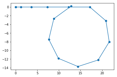
It is also possible, to plot at specific points (yeah, getting there). Let us try for specific set of x,y points, with a constant $\Delta $ u,v set as below. This is direct extract of our X,Y we got from get_x_y earlier.
import matplotlib.pyplot as plt
import numpy as np

x = [0,0,1.225,3.675,7.35,12.25,17.15,20.8747296,21.63742781,19.07222661,14.40965867,9.886368107,7.672187372,8.82926384,12.80254538]
y = [0,0,0,0,0,0,0,-3.183769683,-8.024047717,-12.19894206,-13.7057467,-11.82164413,-7.450442506,-2.689016874,0.178566394]
u = [0.07]*15   # 15 u points caz, there are 15 x points
v = [0.02]*15   # 15 v points caz, there are 15 y points

plt.quiver(x, y, u, v, scale=1)
plt.show()

Aha, we are already getting somwhere. Now think of the arrow direction. What would we want to indicate at any instant (or point location)?
We want the arrow to
- point towards its next location at next instant, so we get a directional sense of trajectory
- represent displacement by its length, so giving a sense of how much "weight" it exits at any point to be at next point
Might be confusing, but this could be easily achieved, just by taking relative displacement values $(dx,dy)$ at each instant, by taking difference of values at that instant from previous one.
Note, the relative displacement values should be scaled down, because, their difference could be easily greater than unit distance in both X or Y direction.
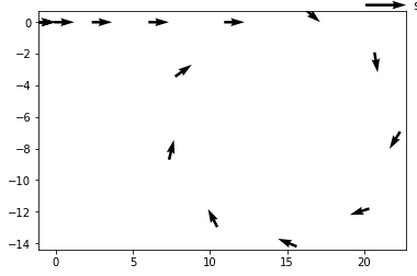
Check out below snippet. We take the relative displacement at every instant and weigh it down, so arrows are shortened, but still representative of relative displacement at that instant.
import matplotlib.pyplot as plt
import numpy as np

x = [0,0,1.225,3.675,7.35,12.25,17.15,20.8747296,21.63742781,19.07222661,14.40965867,9.886368107,7.672187372,8.82926384,12.80254538]
y = [0,0,0,0,0,0,0,-3.183769683,-8.024047717,-12.19894206,-13.7057467,-11.82164413,-7.450442506,-2.689016874,0.178566394]

u = [0]
v = [0]
for each_abs_index in range(1,len(x)):
    dx = x[each_abs_index] - x[each_abs_index-1]  # relative displacement
    dy = y[each_abs_index] - y[each_abs_index-1]
    u.append(dx/75)   # scaling it down
    v.append(dy/75)

plt.quiver(x, y, u, v, scale=1)
plt.show()

Voila. We arrived at the desired visualization. Actually ours is better, because length of arrow is also representative of how much displacement happening at an instant to result in next location.
Let us compare our solution with that of Udacity's.

Now, all that is left is to supply accordingly x,y to above snippet, wrap it as a function and check again.
from solution_parthi2929 import Vehicle, get_derivative_from_data, get_integral_from_data
from math import pi

def get_speeds(data_list):
    t = [row[0] for row in data_list]  # time 't'
    z = [row[1] for row in data_list]  # displacement at 't'
    return get_derivative_from_data(z,t)

def get_headings(data_list):
    t = [row[0] for row in data_list]  # time 't'
    y = [row[2] for row in data_list]  # yaw rate at 't'
    return get_integral_from_data(y,t)

def get_x_y(data_list):
    t = [row[0] for row in data_list]
    z = [row[1] for row in data_list]
    yr = get_headings(data_list)

    # relative displacement derivation
    rel_z = [0]
    for i in range(1,len(data_list)):
        delta_z = data_list[i][1]-data_list[i-1][1]
        rel_z.append(delta_z)

    # create our vehicle for test drive to generate X,Y
    v = Vehicle()

    for each_time_index in range(len(t)):
        v.drive_forward(rel_z[each_time_index])      # feeding relative displacement now..
        v.set_heading(yr[each_time_index]*(180/pi))

    X_Y = v.get_trajectory()
    return list(X_Y)[1:]

def show_x_y(data_list):
    """
    Visualization, just implemented
    """
    X_Y = get_x_y(data_list)
    X = [row[0] for row in X_Y]  # get the X separately from X_Y
    Y = [row[1] for row in X_Y]  # get the Y separately from X_Y
    U = [0]
    V = [0]
    for each_abs_index in range(1,len(x)):
        dx = X[each_abs_index] - X[each_abs_index-1]  # relative displacement
        dy = Y[each_abs_index] - Y[each_abs_index-1]
        U.append(dx/75)   # scaling it down
        V.append(dy/75)
    plt.quiver(X, Y, U, V, scale=1)
    plt.show()
    return
from helpers import process_data

data_list = process_data("trajectory_example.pickle")

show_x_y(data_list)